
37 Time Estimation
Estimates have a huge influence on a project and are a large source of project risk. Watch the video on time estimates to learn about how estimates are used for project planning.
| Top-down estimation | Also referred to as macro, estimation methods are used to determine if a project is feasible, to calculate funding requirements, and to determine the resources needed to complete a project. These methods are not extremely accurate but provide a relatively fast way to make an estimate of the time and costs required for a project. |
| Bottom-up estimation | Also referred to as micro, estimation methods are used to provide a detailed, and more accurate, estimate and are usually derived from the detailed list of work packages or activities found in the work-breakdown structure. |
As the video mentions, all estimates contain risk. If estimates are too low, then a project will take more time and money to complete than what was budgeted. Obviously, a bad situation. If estimates are too high, then a project will take less time and money than originally estimated. This might seem to be a desirable situation, but good project managers will realize that estimates that are too high will cause an organization to over allocate resources to a project, thereby preventing other projects from being pursued due to organizational resource shortages. Therefore, it is important to have the most accurate estimates possible. The project team needs to understand the value of accurate estimates and avoid the natural human tendency to pad estimates. Once unbiased estimates for a project have been generated, the project manager can calculate what time buffers and budgetary reserves should be added to the project plan to deal with uncertainty.
Accuracy of Estimates
Prior to project authorization, estimates for project cost need to be given, but these estimates can be rough estimates. As the project progresses, more definitive estimates will be needed and can be generated.
PMI defines the following ranges for estimates:
- Rough Order of Magnitude (ROM). ROM estimates are made at the initiation of the project and can be +/- 50 percent from the actual or final cost.
- Budget Estimate. Budget estimates are used in project planning and can be within a range from -10 to +25 percent from the actual or final cost.
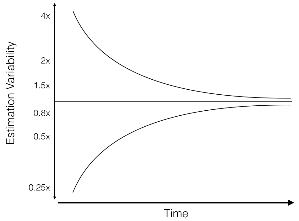
- Definitive Estimate. Definitive estimates are generated as the project progresses and the variability of the estimate is reduced (see Figure 5-4). Definitive estimates are within a range from -5 to +10 percent from the actual or final cost.
Top Down (Macro) Estimation
Top-down, or macro, estimation methods allow for a quick estimate of project costs based on historical information.
Analogous Estimating
Analogous estimating uses information from a previous project to estimate the cost of completing a similar project in the future. This provides a quick estimate, but should be used with caution. Analogous estimating only works when comparing projects that are similar in scope and will be completed in similar conditions.
For example, a small IT business developed a website for a local restaurant for which they charged $4000. Another restaurant approaches the IT firm and asks for a rough cost estimate for a similar site. The IT firm can tell the second restaurant that such work will cost approximately $4000. Of course, the caveat is that this second website will have a similar number of pages, functions, and graphics as the first site.
The advantage of analogous estimating is that it allows for a very quick estimate to be provided for a customer. If in the example above, the second restaurant had only budgeted $200 for a website, they would have quickly determined that they have not budgeted enough, and the IT firm would be able to quickly determine that this is not a serious customer. However, if the second restaurant is okay with this approximate price, the IT firm can work with the restauranteur to develop a detailed cost proposal.
Analogous estimating, is not accurate if:
- The projects differ in scope.
- There is a difference in the conditions under which the work will be performed.
- There is a difference in the cost of resources (materials, labor).
Parametric Estimating
Parametric estimates, also called the ratio method, uses historical information or industry benchmarks as the basis for making an estimate. Parametric estimates are made by multiplying the size of a project by an established cost per unit.
| Cost Estimate (Union Labor) | Cost per Square Foot |
| Labor and Materials | $234.09 |
| Contractor Fees (GC, Overhead, Profit) | $58.52 |
| Architectural Fees | $26.34 |
| Total Building Cost (per Square foot) | $318.95 |
| Cost Estimate (Open Shop) | Cost per Square Foot |
| Labor and Materials | $217.51 |
| Contractor Fees (GC, Overhead, Profit) | $54.38 |
| Architectural Fees | $24.47 |
| Total Building Cost (per Square foot) | $296.36 |
Table 5‑1: Hospital construction costs – Data from Reed Construction (http://www.cmdgroup.com/) 2014.
For example, industry data is available for the per square foot construction cost for many types of buildings. An architect can use this information to make a parametric estimate by multiplying the cost per square foot by the size of any new building being considered. If an organization wants to build a new hospital using union labor, a rough estimate of the construction cost can be calculated using the information in Table 5.1: 20,000 ft² clinic × $318.95/ft² = $6,379,000. The organization can then use this estimate as an approximate cost and start securing the money for the project. Once the funding is secured, an architect can develop a complete plan and produce a more accurate project budget, using a bottom-up estimation method.
Learning Curves
Projects that require an activity to be repeated several times throughout the project will benefit from a so-called learning curve. Learning curves, also known as improvement curves or experience curves, are important when labor is one of our main resources.
Consider a large construction project for a new highway. The first hundred feet of highway may be fairly slow to complete. But as workers become more experienced, and figure out better ways to organize their work, the time required to construct the next one hundred feet of new highway will be less.
Learning curves were first observed in aircraft production and are also used heavily in operations management. Each time production doubles, a learning rate can be calculated. See Table 5.2 for the calculation of a learning curve. When output doubles, from the first screen installed to the second, a learning rate is calculated. Another learning rate is calculated when the output doubles from the second screen installed to the fourth, and so on. The average learning curve can then be calculated. Later, if this company is contracted to install projector screens as part of a project, they can use this learning curve in their labor estimates.
There is a limit to the improvement of a learning curve. Eventually, the learning curve will “bottom out” and no more improvement gains can be achieved.
Table 5-2
| Number of
screens installed |
Time to install
projector screen |
Learning Rate | |
| 1 | 500 | ||
| 2 | 440 | 88.0% | |
| 3 | 420 | ||
| 4 | 400 | 90.9% | |
| 5 | 390 | ||
| 6 | 380 | ||
| 7 | 370 | ||
| 8 | 360 | 90.0% | |
| 9 | 355 | ||
| 10 | 350 | ||
| 11 | 345 | ||
| 12 | 344 | ||
| 13 | 342 | ||
| 14 | 340 | ||
| 15 | 339 | ||
| 16 | 338 | 93.9% | |
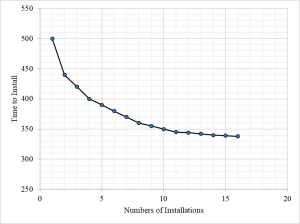
| Average | 90.7% | Data from Table 5-2 shown on graph 5-5. Notice that the longer production occurs, the less improvement from one installation to the next. |
However, there are several things that can be done to extend and improve the slope of a learning curve:
- Incentivize workers to improve the processes they are using to complete their tasks. These incentives are “built in” for companies that are employee owned, where employees share in the reward if profits increase.
- Make investments in new technology and equipment.
- Invest in training and education for new workers, so they are not “learning on the job.”
- Give workers the flexibility to make changes to how materials are sourced, delivered, and organized.
- Re-engineer the deliverables so they are easier to produce.
Learning curves usually hold if the work is continuous. If there is a break in the work, gains in productivity when work resumes will not be as great as if the work had continued uninterrupted.
Bottom Up (Micro) Estimation
Bottom up, or micro, estimation techniques are used when the project is approved or is very likely to be approved. Bottom up estimation techniques generate estimates for individual work packages or sub-deliverables, which are then summarized to reflect total costs. Bottom up estimates are more accurate, detailed and take more time to generate. Instead of relying on historical information, bottom-up estimates rely on people with experience who can provide time and cost estimates for a particular work package or sub-deliverable.
These basic guidelines should be followed when generating bottom up estimates:
- Have people familiar with the work make the estimate.
- If possible, use several people to make estimates.
- Estimates should be based on normal conditions and a normal level of resources.
- Estimates should not make allowances for contingencies.
The project manager or team will add buffer times and contingency funds to the project after estimates are collected and analyzed.
Single Point Estimate
Single point estimation is an estimate obtained from just one estimator. This can work well with experienced estimators and work packages that are straight forward. Single point estimates are quick to generate and summarize in a project plan. The risk with single point estimates is that the estimator will overlook some aspect of the work and inadvertently provide an inaccurate estimate.
Three-points estimate
Instead of asking an estimator for just one estimate, a three-points estimate asks the estimator to provide three-time estimates for each activity:
- An optimistic time estimate (if all goes well, what is the shortest time period one could realistically expect for the completion of this activity?). This will be designated in calculations as a.
- The most likely time estimate (if all goes normally, what is the average time one would expect it would take for an activity to be completed?). This will be designated in calculations as m.
- A pessimistic time estimate (if work goes poorly, what is the longest time period one could realistically expect for the completion of this activity). This will be designated in calculations as b.
These three estimates can be used as inputs to calculate an estimated time for the activity or work package to be completed, either through a simple average or through a weighted average know as T_e, where T_e=(a+4m+b)/6.
How to Improve Project Estimates
Text Attributions
This chapter of Project Management is a derivative the following texts:
Essentials of Project Management by Adam Farag is licensed under a Creative Commons Attribution-NonCommercial-ShareAlike 4.0 International License, except where otherwise noted.
